An electronic payment system requires record-keeping and informationprocessing technologies for transaction clearing and verification purposes. However, from the society’s point of view, the installment and operation of such technologies incur some resource cost. Hayashi and Keeton (2012) refer to this resource cost as the “social cost” of using electronic payment methods and distinguish it from “private cost” that includes the fees imposed by one party to another. This social cost has the distinct feature of being composed largely of fixed costs that do not rely on the frequency or value of the transactions. Once the electronic recordkeeping and information-processing devices are installed at a substantial cost, electronic payment services could be provided with trivial marginal cost.
Considering the high social cost incurred in the installment of electronic payment technology, it is quite natural to ask how the social cost should be allocated. However, to the best of our knowledge, no study has thoroughly addressed this question. Most recent studies on electronic payment systems have focused on issues related to private cost (
This paper examines an optimal allocation of the social cost for an electronic payment system by incorporating a standard Ramsey approach into a dynamic general equilibrium model where money is essential. Specifically, we adopt a standard search-theoretic monetary model augmented with distribution of wealth. We consider wealth heterogeneity across agents to capture economy of scale in the use of an electronic payment system. At the beginning of a period, each agent becomes a buyer, a seller, or a non-trader with some probability. Each buyer is then relocated randomly to match with a seller. After the realization of such relocation shock, a buyer determines whether to carry cash or to open a checking account for subsequent pairwise trade. Carrying cash incurs disutility cost because of the inconvenience and the risk of loss. A buyer can also pay in cash by withdrawing the amount from her checking account where, for simplification, cash-withdrawing cost is assumed to be the same as its carrying cost. A buyer opening a checking account can also use an electronic payment system by shouldering its fixed installment cost.
As agents cannot commit to their future actions and trading histories are private, all trades in a pairwise meeting are
We use the model to examine an optimal allocation of the social cost for an electronic payment system. Our Ramsey problem is a standard one; to maximize social welfare, the government chooses a policy on the allocation of the social cost for an electronic payment system across buyers and sellers who use the system in pairwise trades. Under the assumed buyer-take-all trading protocol, this problem is transformed into that of choosing a tax scheme on the beneficiaries (
The choice of taxation on a buyer’s labor or consumption not only has an intensive-margin effect on the terms of pairwise trade for a given cost per electronic transaction but also an extensive-margin effect on the choice of means of payment. The welfare implications of these two effects depend crucially on a nondegenerate distribution of wealth and economy of scale in the use of an electronic payment system.
With regard to the intensive-margin effect, labor taxation turns out to have a lump-sum feature in the sense that it does not affect quantity consumed in exchange for money transferred electronically, whereas consumption taxation turns out to be distortionary in the sense that it affects quantity consumed in electronic transactions. Hence, labor taxation favors relatively poor agents whose consumption is sufficiently small, whereas consumption taxation favors relatively rich agents whose consumption is sufficiently large. As the tax rate on labor increases (or the tax rate on consumption decreases), the difference between the average quantity of good consumed by buyers and that produced by sellers decreases.
Labor taxation also has an extensive-margin effect on the choice between electronic and cash payment, which then affects the cost per electronic transaction via an economy-of-scale channel. In particular, the frequency of electronic transactions is shown to increase with the tax rate on labor. When the tax rate on labor is zero for a given cost per electronic transaction, relatively poor buyers with sufficiently high marginal utility of consumption are willing to pay in cash rather than use electronic payment even if the cash-withdrawing cost exceeds the tax burden associated with the use of electronic payment. However, as the government increases the tax rate on labor, a greater number of poor buyers prefer electronic payment to cash payment, yielding economy of scale in the use of an electronic payment system. This economy of scale decreases per transaction cost of electronic payment, consequently enhancing both intensive-margin and extensive-margin effects of labor taxation.
These results imply that overall transaction cost, including welfare loss because of resource cost for an electronic payment system (which is raised in the form of labor taxation and distortionary consumption taxation) and cash-withdrawing cost, decreases with the tax rate on labor. As a result, the unity tax rate on labor (or zero tax rate on consumption) yields an optimal allocation of the social cost for an electronic payment system.
The paper is organized as follows. Section II describes the model economy. Section III defines a symmetric stationary equilibrium. Section IV formulates the Ramsey problem for the benevolent government and examines an optimal allocation of the social cost for an electronic payment system. Section V summarizes the paper and provides several concluding remarks.
The background environment is in line with a standard random matching model of money (
Time is discrete. There are
Three exogenous nominal quantities describe the stock of money: upper bound on individual money holdings, size of the smallest unit of money, and average money holdings per type of agent. We normalize the smallest unit to be unity so that the set of possible individual money holdings consists of integer numbers, namely, M={0, 1, 2, ...,
At the beginning of each period, each island is randomly connected to another island, which can be interpreted as a preference shock in the sense that an agent becomes a buyer or a seller with an equal probability 1/
In a newly migrated island, each buyer is matched with a seller for a pairwise trade. Trading histories are private and agents cannot commit to future actions; thus, any possibility of credit trades is ruled out and a medium of exchange is essential (see, for instance, Kocherlakota 1998; Wallace 2001; Corbae
In a pairwise trade, a buyer makes a take-it-or-leave-it offer (
Transactions via an electronic payment method require the installment and operation of an electronic payment system, for which the government (
In order to provide debit-card service to the society, the government should raise resources Ω to pay for the fixed cost incurred in installing the debit-card payment system. First, unlike a representative agent model such as Lagos and Wright (2005), our model allows for wealth heterogeneity across agents, including those with no money. Hence, allocating the social cost for the debit-card payment system in a lump-sum fashion is not feasible. Under the assumption that cash-withdrawing cost from a checking account is the same as its carrying cost, taxation on cash traders is not feasible because they would then evade taxation by carrying around cash, which is not in the government information system. However, the government is notified of debit-card transactions because they are cleared through the debit-card payment system operated by the government. Therefore, the government can effectively collect the required resources from debit-card traders.
Specifically, according to the widespread agreement on fixed cost per debit-card transaction (see, for instance, Wang 2010), the government is assumed to raise resource cost Ω by levying
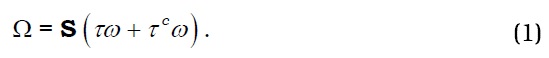
Here, S denotes the frequency of debit-card transactions;
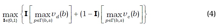
For a given (Ω,
For a type-

where
After a pairwise trade, a buyer returns to her home island and the information on each checking account is completely wiped out.3 An agent goes on to the next period with end-of-period money holdings.
1As shown by Head and Kumar (2005) and Rocheteau and Wright (2005), for instance, this trading protocol can mimic an allocation in a competitive market (or a market with competitive price posting). Suppose that type-n buyers in village j are matched collectively with type-(n+1) sellers in village k and then they trade in a competitive market (or in a market with competitive price posting). An equilibrium allocation would be reminiscent of an allocation with a buyertake-all bargaining, where a buyer has j amount of money and a seller has k amount of money. 2In Section IV, we consider the case in which the proportional cost η is replaced with a fixed cost. We also consider the case in which cash-carrying cost is borne by a seller. 3Note that unsecured credit transactions are available and money is inessential if the government is assumed to have an inter-temporal record-keeping technology rather than an intra-temporal one.
We study a symmetric (across “islands” or specialization types) and stationary equilibrium. For a given (Ω,
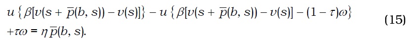
Consider a generic pairwise meeting between a buyer with

That is, Γ(
where


Let


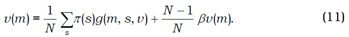
Now, let

where
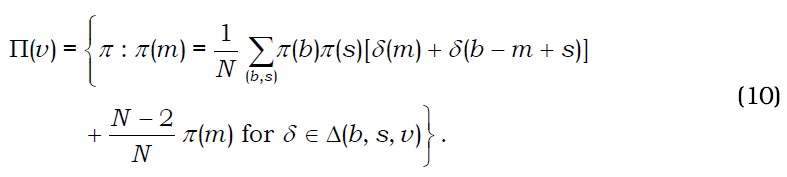
Now we can describe the evolution of wealth distribution induced by pairwise trades as follows:

The first probability measure on the right-hand side of (10) corresponds to pairwise trades, whereas the second corresponds to all other cases.
Noting that in (9),
Finally, let

Definition 1:
The existence of a symmetric stationary equilibrium for some parameters is a straightforward extension of the existence results in Zhu (2003) and Lee
4Without the loss of generality, we can disregard the case in which a fraction of p is paid in cash and the remainder using a debit card because once a debit card is used, cost per debit-transaction (ω) is imposed regardless of the amount of debit-card transaction.
We now examine an optimal allocation of the social cost for an electronic payment system using a standard Ramsey taxation approach.
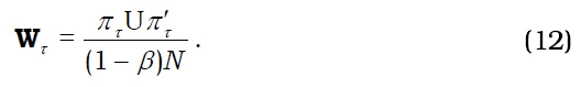
In order to formulate a Ramsey problem for the benevolent government as a provider of debit-card payment services, we first define welfare as the lifetime expected discounted utility of a representative agent before the assignment of wealth according to a stationary distribution. Let W

Here, the element in row

with
Under the buyer-take-all trading protocol, the benefit principle is implementable in the sense that the social cost for the debit-card payment system is borne by its beneficiaries (

where
Now the Ramsey problem for the government is to choose the tax rate on labor (
Definition 2:
In order to compare the magnitude of welfare loss across different policies, we calculate the welfare cost of
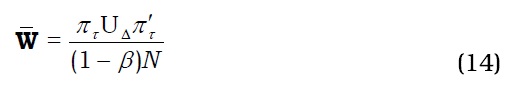
where is the welfare with lump-sum taxation. The element in row

That is, Δ is an additive consumption compensation that makes the welfare with
Although labor taxation (
Labor taxation (

It can be shown that pe105(
This extensive-margin effect will lower per transaction cost (
The above discussion suggests that the effect of
We parameterize the basic environment to solve the model numerically as follows. We first assume
We let
>
C. Labor Taxation versus Consumption Taxation
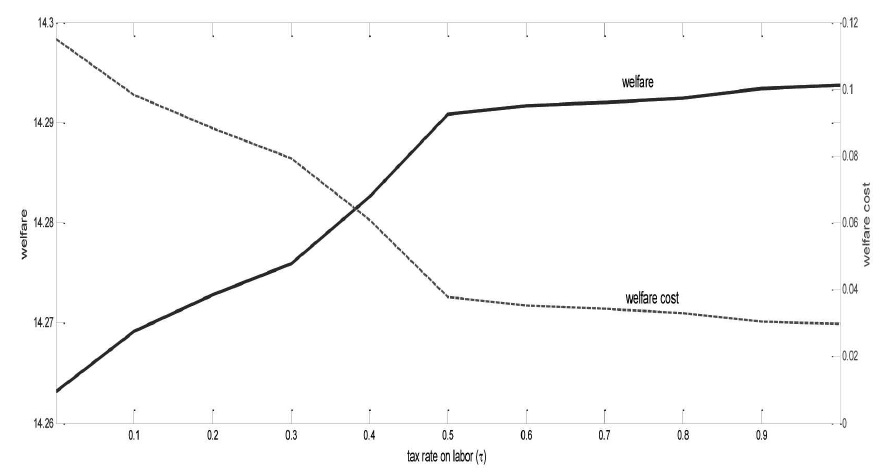
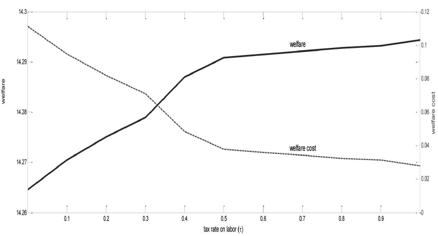
Figure 1 shows welfare level and welfare cost as a function of the tax rate on labor (
The underlying mechanism that renders the unity tax rate on labor (or zero tax rate on consumption) optimal can be explained in terms of (i) its intensive-margin effect on the quantity consumed in exchange for money transferred via a debit card for a given cost per debit transaction and (ii) its extensive-margin effect on the choice of means of payment between debit card and cash, which affects the cost per debit transaction. The welfare implications of these two effects hinge on a nondegenerate distribution and economy of scale in the use of debit-card payment system.
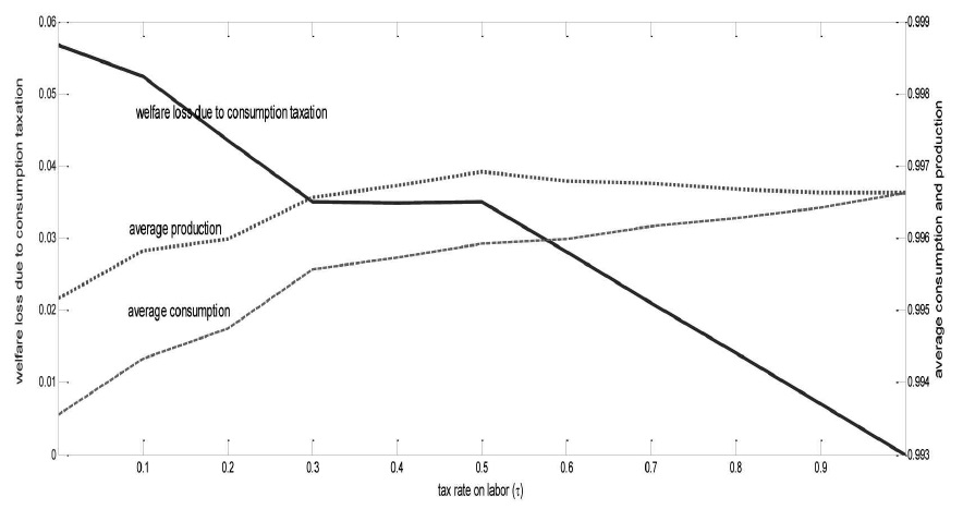
First, with regard to the intensive-margin effect, a higher tax rate on labor implies relatively low tax rate on consumption, thereby mitigating consumption distortion. Hence, the higher the tax rate on labor (consumption), the more favorable to the relatively poor (rich) whose consumption is sufficiently small (large). Figure 2 shows that the gap between the average quantity of good consumed by buyers and that produced by sellers shrinks as the tax rate on labor increases. As a result, welfare loss due to distortionary consumption taxation decreases and eventually converges to zero as the tax rate on labor approaches 1.
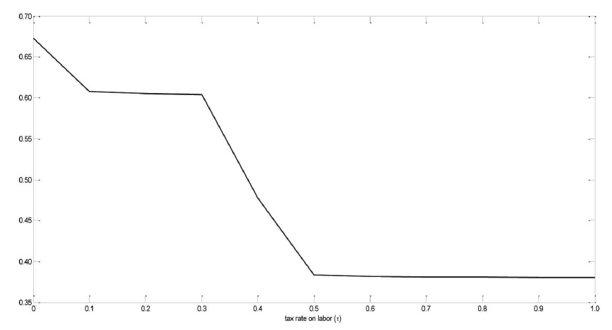
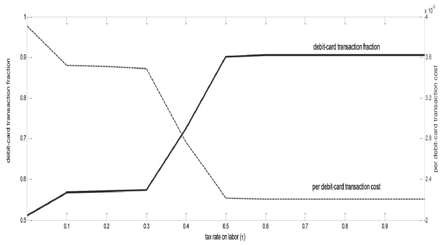
Second, a higher tax rate on labor also has an extensive-margin effect on the choice of payment method. Figure 3 shows that the frequency of debit-card transactions (S) increases with
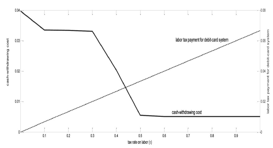
Third, Figure 5 shows that the total cost of withdrawing cash decreases with the tax rate on labor. This is because the frequency of cash transactions decreases as
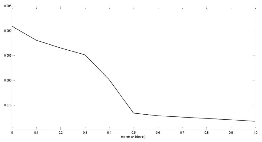
In sum, Figure 6 shows that overall transaction cost, including welfare loss due to social cost for the debit-card payment system (which is raised in the form of labor taxation and distortionary consumption taxation) and cash-withdrawing cost, decreases with the tax rate on labor. This immediately implies the results shown in Figure 1.
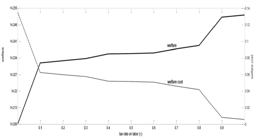
Finally, we check the robustness of our main results in different settings. We first consider the fixed cash-carrying cost for sellers. That is, a seller accepting cash incurs a fixed handling cost
As another robustness check, we consider the case in which the cash-withdrawing cost for a buyer is fixed, whereas the cash-carrying cost for a seller is proportional. That is, withdrawing cash incurs a fixed cost for a buyer, whereas cash-handling cost for a seller increases with the amount of cash transaction at a rate of . In computing a stationary equilibrium for this case, we again choose (, ) to make the model fit the data. The model parameterized with (
5If the social cost for debit-card payment system is raised by imposing a lump-sum tax on each agent, all trades are made using debit cards, and trading behaviors are not affected. However, as discussed in Section II, lump-sum tax cannot be forced effectively in our model. 6Consumption compensation is calculated as an addition to the consumption with τ-policy rather than as a multiple of consumption with τ-policy, because consumption is zero in some pairwise meetings. 7Note that the left-hand side of (15) is decreasing in p, whereas the righthand side is increasing in p. The left-hand side is also greater than the righthand side when p is sufficiently close to 0. Hence, (b, s) in (15) is well defined. 8In this type of model, almost all monetary offers are either 0 or 1 if the indivisibility of money is too severe. However, it is not the case in our examples. In addition, M=3 is large enough so that almost no one is at the upper bound in a stationary equilibrium and hence, the result would be hardly affected even if a larger M were assumed. 9Recent empirical studies such as Garcia-Swartz et al. (2006) and Schmiedel et al. (2012) suggest that both buyers and sellers incur cash-carrying cost.
In this paper, we explored an optimal allocation of the social cost for an electronic payment system by incorporating a standard Ramsey taxation approach into an off-the-shelf matching model of money. Our results suggest that economy of scale in the use of an electronic payment technology is enhanced with the tax rate on labor. This then decreases not only per transaction cost of electronic payment and cash-withdrawing cost, but also welfare loss because of the distortionary consumption taxation. As a result, the unit tax rate on labor (or zero tax rate on consumption) yields an optimal allocation of the cost for an electronic payment system.
In order to capture an economy-of-scale channel thoroughly, we here adopt a Trejos-Wright model. Alternatively, we can also consider a rather tractable model such as a version of Lagos and Wright (2005). For the model, tractable distribution of wealth can be generated in many ways, allowing us to obtain a closed-form solution. We believe, however, that even in this case, our main mechanism would still work and the main results would remain intact.
Finally, we focused on an allocation scheme of the social cost for an electronic payment system without considering its implications from the viewpoint of an industrial organization. For instance, we do not deal with the issue on how to impose fees on merchants and consumers by a profit-maximizing card issuer. We leave the generalization of our model to future research, in which private fees together with the resource cost can be explored systematically.