Due to the customer needs of reducing cost and delivery date shorting, prompt change in the production plan became more important.
In the social system or production process of multi periods (or machines or workers) where target processing time exists, idle and delay risks occur repeatedly for multiple periods. In such situations, delay of one process may influence the delivery date of an entire process. In this paper, we discuss the minimum expected cost of the case mentioned above, where the risk depends on the previous situation and occurs repeatedly for multiple periods. There exists an object with some constraints (e.g., due date of production process). These constraints produce a risk and the object occurs repeatedly for multiple periods. This kind of problem is called “a limitedcycle problem with multiple periods” (Yamamoto
Under the condition of uncertainty, the result or efficiency of a period is often controlled not only by the risks of this period but also by the risks generated beforehand. Whether the process (period or seat) satisfies the due time (restriction) usually depends on the state of the process beforehand, as seen in Wright
In particular, in the case of the risk which depends on a situation of a past process (for instance, the case of a production line for a multi period), how to assign machines, workers or jobs to be most efficient and economical is a problem (optimal assignment) in load/risk planning (for example, see Bergamashi
Yamamoto
where
This paper considers cases in which the above two risks not only occur in the single period, but also in multiple periods repeatedly. The problem of minimizing the expected cost in such a situation is a limited-cycle problem with multiple periods. The multi period problem could be classified according to whether the periods are independent or not
For this problem, one result is the general form of production rate and waiting time by a station-centered approach as discussed in Matsui
This paper considers the optimal switching frequency to minimize the total expected cost of the production process. In this paper, first, the optimal switching frequency model is proposed. Next, the mathematic formulation of the total expectation is presented. Finally, the policy of optimal switching frequency is investigated by numerical experiments.
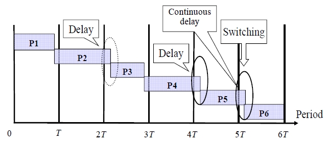
In the production process of multi periods, delay of one process may influence the delivery date of an entire process. We consider controlling the production process by switching the processing rate to a faster one at a given point. The optimal switching problem is when the processing rate should be switched to minimize the total expectation cost. In this paper, we consider the optimal switching point to minimize the total expected cost of the production process. In our considered model, if processing are delay
2.1 The Assumption and Notation
The optimal switching frequency model for the multi limited-cycle is considered based on the following assumptions:
(1) One product is made by a process with n processes.
(2) For i = 1, 2,…, n, the production time of process i is denoted by Ti which is assumed to be exponentially distributed and statistically independent, respectively. The usual processing rate is μ1 , and the emergency processing rate is μ2 .
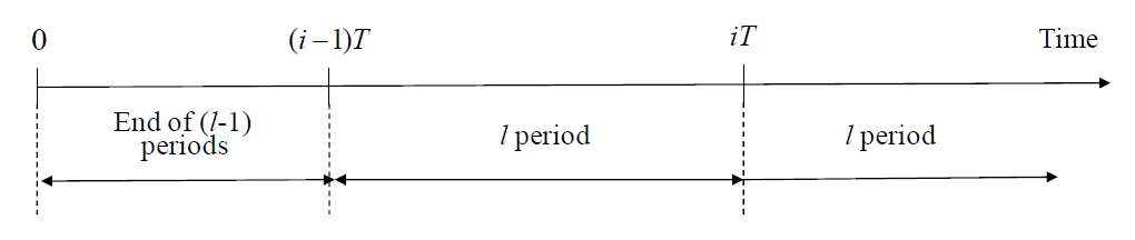
(3) For i = 1, 2,…, n, the target production time of process i is denoted by T, which is set by standard of the process, and the due time of the entire process (n periods) is nT.
(4) k is continuous delay times.
(5) The cost per unit time ( Cs(i) ) occurs when a process is executed before the target production time of the process (i = 1 means before switching and i = 2 means after switching).
(6) The cost per unit time ( Cp(i) ) occurs when a process is executed after the target production time of the process (i = 1 means before switching and i = 2 means after switching).
(7) When
of n periods, the delay cost Cp occurs
(8) When
of n periods, the idle cost Cs occurs.
Some notations are also defined.
For
C (T1, T2, … Tn) : the total cost of the production process.
C(i) : the production cost of period i
Ti : the production time of period i.
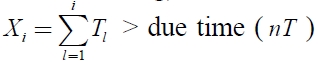
Xi : the production time of i periods
Pr(Xn > nT) : the probability of delay.
Pr(Xn ≤ nT) : the probability of idle.
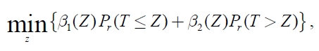
By assumptions mentioned in section 2.1, the object function is set as follows:
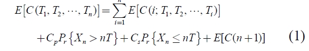
where,
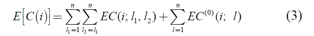
E[C(i; T1,T2,…,Ti)] is the expected cost of period i,
C pP r {X n > nT} is the delayed expected cost,
C sP r {X n ≤ nT} is the idle expected cost,
E[C(n+ 1)] is production cost after due time,
and for
where
In this paper, for
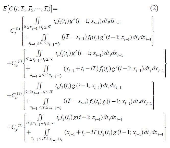
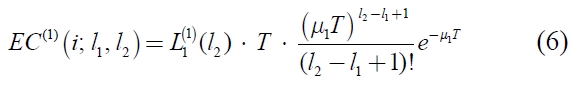
Based on the relation between exponential distribution and Poisson distribution, the terms in equation (1) are given as follows:
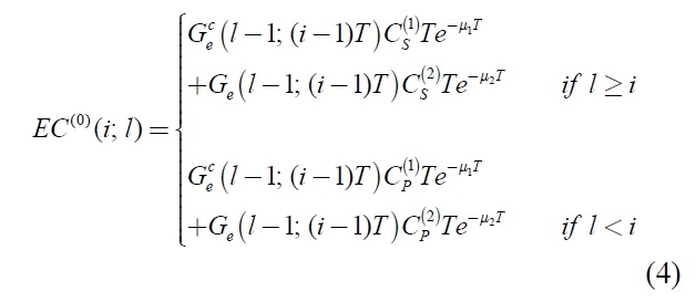
For
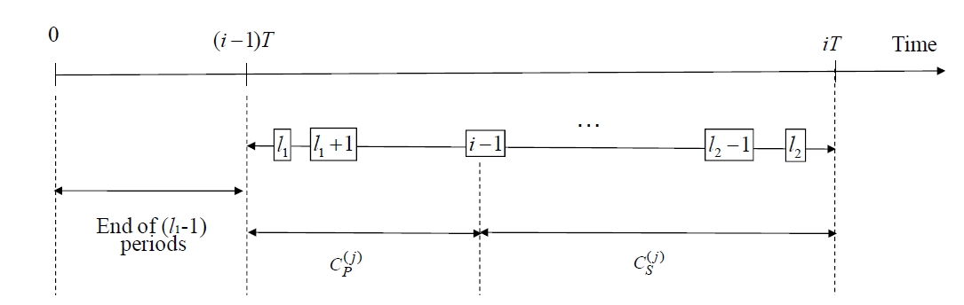
Gc (i; t) : The distribution function of total production costs of period i ended on time t, and process doesn’t exceed k times continuously from period 1 to i (before switching).
gc (i; t) : The probability density function of Gc (i; t) .
G (i; t) : The distribution function of total production costs of period i ended on time t, and process doesn’t exceed k times continuously from period 1 to i (after switching).
g (i; t) : The probability density function of G (i; t)
The probability of period i ended on time t, and process doesn’t exceed k times continuously from period 1 to i, and Xi < t
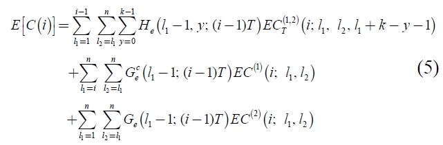
Ge (i; t) : The probability of period i ended on time t, and process exceed k times continuously from period 1 to i, and . Xi < t
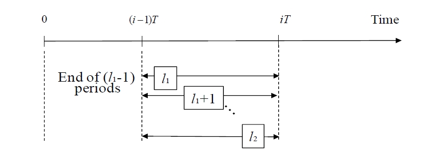
He (i,l; t) : The probability of period i ended on time t, process doesn’t exceed k times continuously from period 1 to i-l-1, and period i-l doesn’t exceed, and period i-l-1 to i all exceed.
Theorem 1:
For
Theorem 2:
For
Theorem 3:
For
Theorem 4:
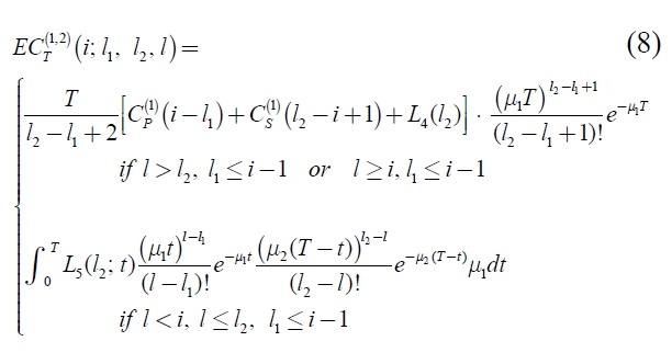
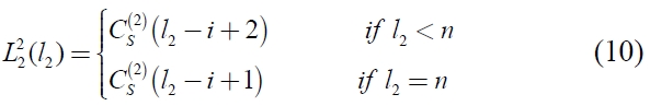
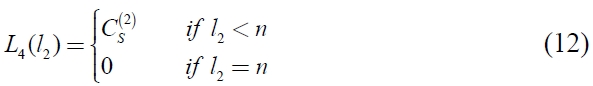
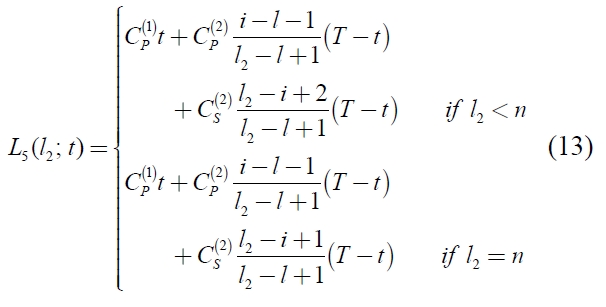
(i) For
(ii) For
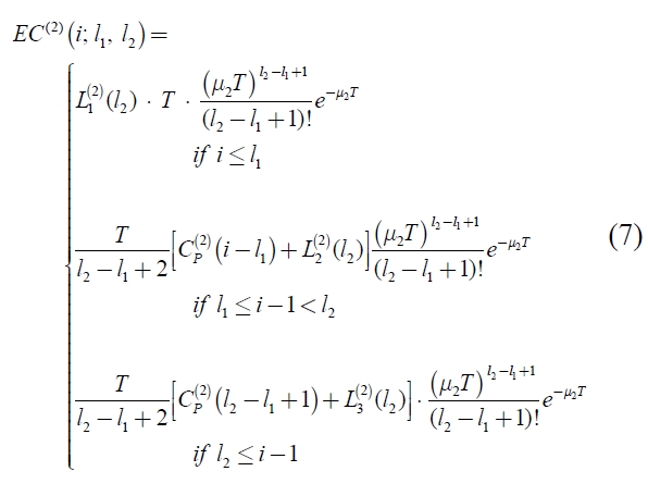
(iii) For
where, for
and

Theorem 5:
For

In this section, we consider the optimal switching times to minimize the total expected cost by numerical experiments, where
We show three cases by production process situations as follows:
(I) Total cost concludes production cost before due time, delay and idle costs.
(II) Total cost concludes production cost (before due time and after due time), delay and idle costs.
(III) Total cost concludes production cost (before due time and after due time).
We can note that (II) is the case of equation (1).
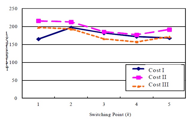
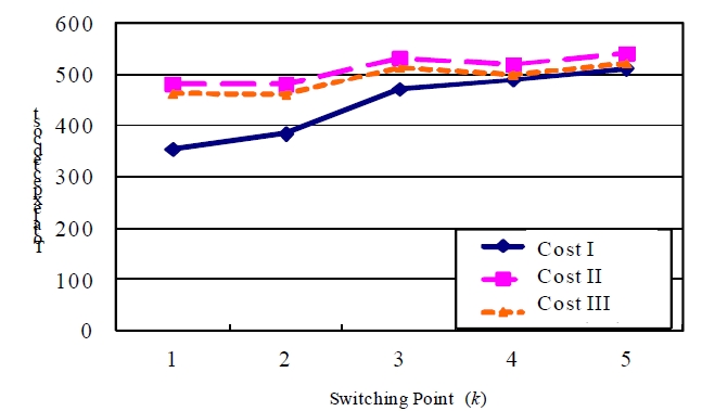
Figure 5 and Figure 6 show the relation of expected costs and switching point
Figure 5 shows the behavior of the optimal switching point by change of continuous delay times (
Figure 6 shows the behavior of the optimal switching point by change of continuous delay times (
From Figure 5 and Figure 6, it also can be noted that optimal switching point
In this paper, we considered the optimal switching point to minimize the total expected cost in limitedcycle problems with multiple periods. First, the optimal switching frequency model is proposed. Next, the mathematic formulation of the total expectation is presented. Finally, the policy of optimal switching frequency is investigated by numerical experiments, and the optimal switching point could be found, too.